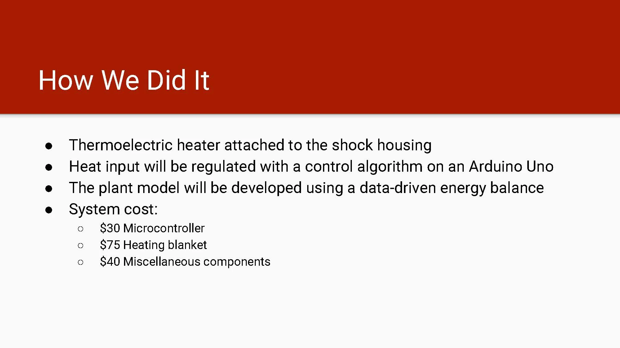
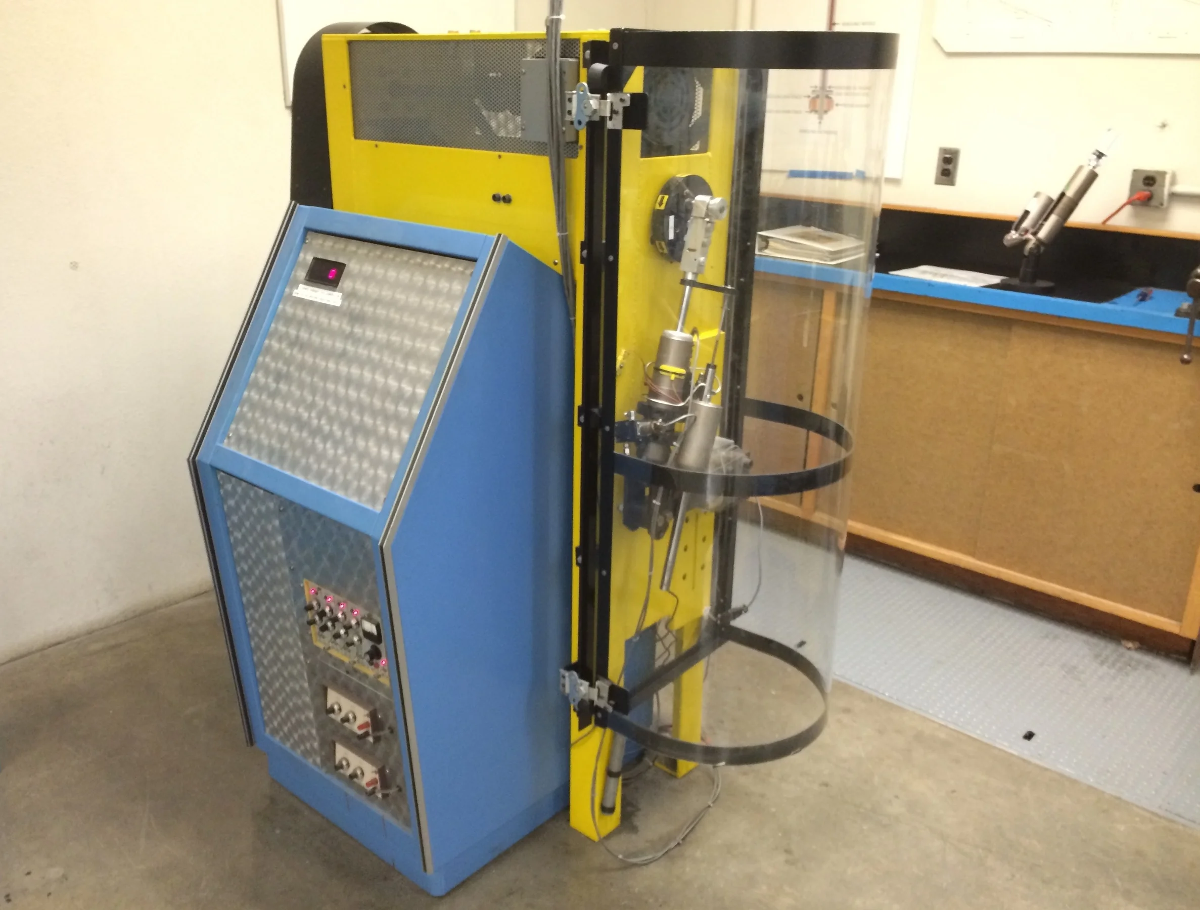
Outside of lab, we made much progress on the modeling and simulation of the entire system. Although there are still some challenges to be overcome, the majority of the controller has been designed in Simulink, and MATLAB functions have been created to estimate the viscous heat generation and convective heat loss as functions of dyno RPM and ambient temperature. Rather than using a first principles model and known empirical formulas as we first attempted, we are now approaching the system with a data-driven model using the known specifications of the motor and the measured force values at different RPM’s. The main goal for next week is to finish designing the controller and modeling the system heat losses so that we can run effective and realistic simulations. Once simulations are complete, we can then begin to order hardware and design the physical heating system.
Thanks for reading!
-The Hot Shocks
INDIVIDUAL THOUGHTS
GRACE
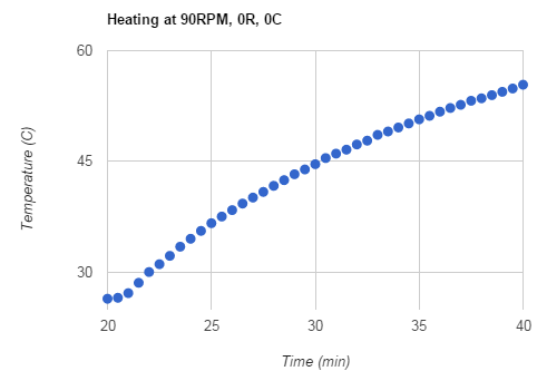
This week I focused on a couple of things. First, I, once again fit the temperature vs. time data to the same y = a + (1 + exp(-x/b))*c curve for the 20W oil at RPMs of 30,60, and 90. For this oil we would postulate that the steady state temperature would be higher for each given RPM than the 10W oil, and it is! Since the oil is more viscous, the motor must put out more force to shear it, so it is inputting more work (and more heat) into the system. Shout out to Couette for helping us predict this result. I found that the steady state temperatures are about 32, 50, and 75 degrees Celsius for RPMs of 30, 60, and 90 respectively.
Second I gave a go at understanding more about the input work into the system. In lab we had talked about using the work done by the motor to characterize the heat added to the system through the shock. This is a great idea, but I thought I’d give a go at simply using our temperature vs. time data to solve for Qin so we could hopefully verify our results. I used the equation Qin + Qout = mcdT to start. I know that the viscosity decreases more or less exponentially with temperature, so I let Qin be modeled by Qin = X*e^(1/T) where X is some parameter to be solved for and T is the oil temperature. Next, I let Qout = Y*(T - Tenv) where Y is the combined heat transfer coefficient and surface area. The mass, m, and heat capacity, c, were previously estimated. Next I used our temperature vs. time data to make a system of equations to solve for X and Y. I used a least squares fit method to find these parameters from the data. I found that for 30, 60, and 90 RPM, the shock dissipates about 14W, 40W and 60W. These values feel a little low to me, so I’ll work with other group members to try to improve these results, or understand the errors.
TURNER
This week I focused on finalizing the energy balance for the shock, which would help Les and Eric tune the gains of the controller by allowing them to accurately simulate the heat transfer processes in the shock. My first attempt involved using the steady state temperature of the shock at different rpm’s to estimate the heat transfer coefficient, h. Assuming radiation to be negligible, I wrote a MATLAB function that, when given the rpm, the steady state temperature of the shock body, and the ambient temperature, outputs the heat transfer coefficient and total convective heat loss. Because the calculations were done for steady state, the idea was to equate the convective heat loss to the viscous heat generation within the shock. The heat transfer coefficient was estimated using empirical relations for the Nusselt number of a cylinder in cross-flow given in Fundamentals of Heat and Mass Transfer by Bergman, Lavine, Incopera, and Dewitt.
However, after using the estimated heat transfer coefficient in simulations, it did not seem to agree with our data, especially in the transient cases. This discrepancy is most likely due to the fact that the velocity used in forced convection calculations is not easily defined in this scenario and because there is no empirical relation that exactly fits the motion of the shock dyno. Because of this, on the suggestion of our GSI, Spencer, we decided to estimate the power input to the shock (via the motor) rather than the convective heat loss. We have received the specifications for the motor being used by the dyno, and now we must make appropriate assumptions and use our data to calculate the power input, and thus estimate the heat generation due to viscous forces within the shock. This work is scheduled to be completed within the next couple days, and I’m excited to see our simulations coming together so we can start working on the hardware in the near future.
LES
I spent most of this past week further developing the model for both the plant and controller. The the system model is fully operational and the open-loop system shows results that are consistent with the data we have gathered in lab, thanks to the heat transfer analysis Turner and Grace have been performing. I’ve begun tuning the closed-loop model but it became apparent this week that this particular type of control problem is a part of what’ is known as bang-bang control theory, so-called because the controller operates solely on its rails, i.e. maximum input or minimum input. In our particular case, we have an Arduino microcontroller that takes in temperature error (e=Tref-T) and uses it to determine a pulse-width modulation (PWM) output to send to the solid-state relay controlling the heater. This is problematic because the temperature error is theoretically unbounded, but PWM duty cycles are fundamentally bounded between 0 and 100%. I was able to linearize the system by bounding the system error and performing a one-to-one linear mapping of error to PWM duty cycle.
The error bounds are consistent with how we expect the shock temperature to behave in real life, and for kP=1 our system response as a first-order closed-loop system should. Unfortunately, once I started tuning the gains of the PID controller, I realized the mapping was no longer bounded appropriately and so I devised a programmatic rebound proportional to the selected value of kP.When I bounded the output of the controller in this manner, the system response no longer changed for different kPvalues, which suggests to me there may be an error in the model somewhere. I will investigate and resolve this issue before next lab, and once I have done so I will begin tuning the kD and kI gains to speed up the response and improve setpoint tracking. I will also update the model to include a rough estimate of internal energy generation from the viscous heating of the shock, and will refine this energy generation term when Turner and Grace have developed a better data-driven model for it.
CHRISTY
In lab this week, I focused on data collection to help our group finalize the heating and cooling characterizations in order to fully develop our model. We followed the same procedure for temperature measurements as last week with the addition of a second thermocouple to measure the interior temperature of oil as well. In order to get a more robust view of our system, I also took twenty minutes of data at 60 RPM to help determine the rate of temperature increase at a middle speed.
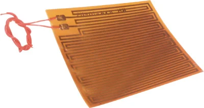
Out of lab, I have been working on answering the questions that Spencer posed last week regarding the safety of the heating blankets and the capability of them to heat the oil quickly enough at a low RPM. Since after twenty minutes at 30 RPM, the max temperature generated was … for the 20W oil, I do not think we will be able to heat the oil rapidly enough with the heat blanket alone. I think that our system will require initial energy input generated by running the shock at 90 RPM for a designated amount of time to prep the system for regulation. This amount of time will be determined based upon our final temperature bounds, but the system should be ran at fully closed compression and rebound to ramp the temperature more quickly. Since Spencer was supportive of my idea to use zip ties to attach the heating blanket, I have begun researching zip ties that can withstand a great enough heat without melting.
ERIC
This week I continued to try and do parameter identification on our original model. In addition to that I have begun to transfer the Simulink block diagrams into Arduino Code. This goes for both the thermostat controller model and a proportional model that I have constructed. In all likelihood the heater we purchase will not have a built in controller. It will simply have two leads and a set impedance. In order to achieve different amounts of heat flux we will have to use H-bridges and a PWM output from the Arduino. Much like a DC motor, this setup will allow us to vary the current sent through the heater. I will map the duty cycle to 100% when the temperature differential is at the extreme (room temp vs 100+ C) and to 0% when the temperatures are within a set tolerance of each other. Once the heater is purchased we can begin testing.
JUSTIN


